Automating Pilot Health Checks with Holt-Winters & Graphite

Recently Netflix announced the release of Kayenta; an open source tool for automating canary analysis they use to ensure their pilot deployments are healthy.

This post outlines how you can achieve something similar with built-in Graphite functionality; we will set up a test server in Docker, populate it with data using Python then build thresholds using the Holt-Winters algorithm.

Context

In my current company we have adopted the use of pilot or "canary" boxes to check releases on production before they are promoted to all customers.

This works by deploying a new release to a small percentage of instances running in production. So if we have 15 boxes running the production release version (v1.4.0) we could spin up 1 new box running the candidate for release (v1.5.2).

A load balancer sitting outside these instances would then direct a percentage of traffic to the pilot box. If it is using round robin in our above example 6.25% of traffic will be directed to the pilot box. Users are frequently "pinned" to either a production or pilot type box after being routed to ensure they get a consistent experience.

The reason we do this is to ensure a release is stable without having to deploy it to 100% of users at once. By rolling out a pilot release to a small percentage of users we can run it overnight checking that there are no errors being logged, issues reported by customers or misbehaving metrics.

Initially however; the checks we do are manual, with developers and support staff looking at graphs of metrics to assess the health of a release before either rolling it out or rolling it back.

What we'll do below is set up a process for automating these checks based on comparing pilot metrics to the baseline production release.

What is Graphite?

Graphite is part of a set of tools frequently used for the collection and display of metrics gathered from a series of components. In the docker container I'm using in the next section there are 3 main components:

• StatsD
  • Used for gathering & aggregating metrics from components.
  • It's responsible for pushing metrics from an instance to the Carbon database.
• Carbon
  • Used to store metrics sent from StatsD.
  • Can also be sent statistics directly, as we'll be doing later.
• Graphite
  • Web application for viewing metrics.
  • This is where we will be building queries against the data.

Metrics sent to Carbon tend to have 3 things:

• A "bucket" or name of the metric, e.g: api.cpu.baseline
• A value, e.g: 52
• A unix timestamp (seconds from epoch), e.g: 1526132128

The packets we'll be sending to Carbon look like this:

api.cpu.baseline 52 1526132128
api.cpu.baseline 49 1526132129
api.cpu.baseline 46 1526132130

Setting up our test environment

We'll use Docker to set up a quick test environment where we can demostrate using Holt-Winters against a running Graphite instance.

To start we'll need Docker Community Edition installed & setup locally. This only supports Windows 10 Professional/Enterprise or Windows Server so if you're using Windows 10 Home then use the Docker Toolbox instead.

Alternatively you could instead use Azure Container Instances, which allow you to run single containers in the cloud with minimal set up. See here for a recent blog post explaining the setup.

Next we'll download our base image, called graphite-statsd. To do this, on the command line run:

docker pull hopsoft/graphite-statsd

This will download the image ready for us to run. This particular image has everything we will need to ingest and view metrics.

Finally, we need to run the container itself:

docker run -d --name graphite --restart=always \
           -p 80:80 -p 2003:2003/udp \
           hopsoft/graphite-statsd

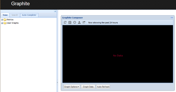
This starts a new container with the graphite image and exposes 2 ports: TCP 80 (Which allows us to use the Graphite web application) and TCP 2003 (This is the Carbon plaintext port we'll send data to). If you open http://127.0.0.1 in your browser you should see the Graphite dashboard:

Pushing our test data

Now we've got a container set up and running, we need to populate it with 2 series of data. The first, api.cpu.baseline, will represent our current production boxes running the stable version of our software. The second, api.cpu.pilot, will represent the new pilot boxes running the release candidate.

Below is the script I used to generate the test data; it randomly creates 2 series with 10 hours worth of metrics, with the pilot being slightly higher on average.

import socket
import time
import random


CARBON_SERVER = "127.0.0.1"
CARBON_PORT = 2003
SERIES_LENGTH = 36000  # 10 hours in seconds


class CarbonConnection():
    """Disposable object for managing a connection to Carbon"""

    def __init__(self, ip, port):
        self.ip = ip
        self.port = port
        self.sock = socket.socket()

    def __enter__(self):
        self.sock.connect((self.ip, self.port))
        return self

    def __exit__(self, type, value, traceback):
        self.sock.close()

    def send_stat(self, bucket_name, value, timestamp):
        message = '%s %i %d\n' % (bucket_name, value, timestamp)
        print('Sending message:\n%s' % message)
        encoded = message.encode("utf-8")
        self.sock.sendall(encoded)


def generate_random_series(points_to_generate, lower_bound, upper_bound):
    series = []
    for i in range(0, points_to_generate):
        series.append(
            random.randint(lower_bound, upper_bound)
        )
    return series


def current_timestamp():
    return int(time.time())


baseline_series = generate_random_series(SERIES_LENGTH, 40, 50)
pilot_series = generate_random_series(SERIES_LENGTH, 40, 55)
starting_timestamp = current_timestamp() - SERIES_LENGTH

with CarbonConnection(CARBON_SERVER, CARBON_PORT) as cc:
    for i in range(0, SERIES_LENGTH):
        timestamp = starting_timestamp + i
        cc.send_stat("api.cpu.baseline", baseline_series[i], timestamp)
        cc.send_stat("api.cpu.pilot", pilot_series[i], timestamp)

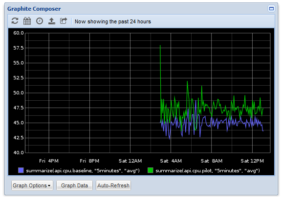
Once this has finished the data we can display it on Graphite by loading it in our browser at http://127.0.0.1 -> "Graphite Composer" -> "Graph Data -> "Add".

In the metric box enter summarize(api.cpu.*, "5minutes", "avg"), click "OK" and the graph should then look a little something like this:

Building our thresholds

Now we have some data set up, we can start looking at using Holt-Winters to build thresholds.

Holt-Winters is an algorithm that allows us to create confidence bands around a set of time series data, and is supported out of the box in Graphite. These bands will act as a set of upper and lower thresholds based on the production CPU that our pilot CPU should fall inside to be considered healthy.

To build our thresholds, firstly open Graphite and go to "Graphite Composer" -> "Graph Data -> "Add"

Add the metric:

summarize(api.cpu.baseline, "5minutes", "avg")

This will display a smoothed version of our baseline graph. Click "OK"

Click "Add" again and set this metric:

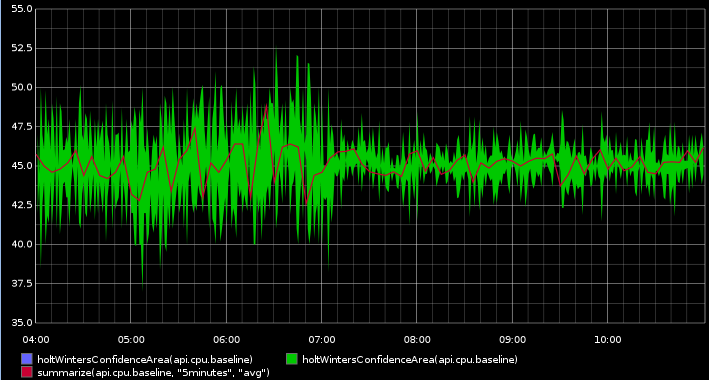
summarize(holtWintersConfidenceBands(api.cpu.baseline, 10), "5minutes", "avg")

This will generate 2 new metrics; the upper and lower confidence bands of our data. If you click "OK" and return to the graph, you should see something like this:

The red line is our production cpu baseline metric; the green and blue lines are thresholds based on the range of values over time in that series. As you see the production cpu sites comfortably inside those bands.

What these thresholds are saying is "If the metric sits inside these bounds, it's comparable to production".

Now let's replace the original baseline metric with our pilot metric:

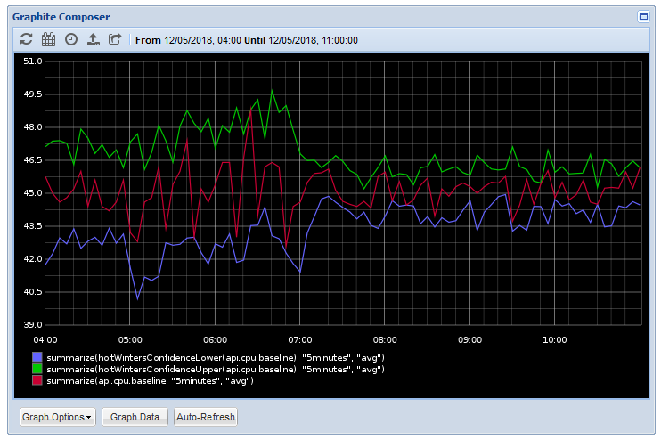
summarize(api.cpu.pilot, "5minutes", "avg")

And look at the graph again:

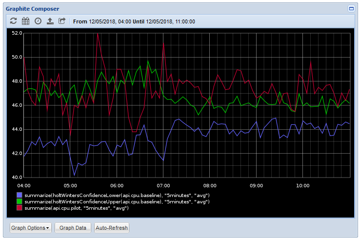
You can see now that the red line, representing our pilot CPU, exceeds the thresholds set, indicating that the pilot box is frequently using more CPU than the production box.

Alerting on the thresholds

So now we have a way to visually identify when a pilot metric strays outside of acceptable bounds when compared to production, we need to come up with a Graphite metric that can be used for alerting.

To do this, firstly remove all metrics from the graph data and replace with this single one:

removeBelowValue(
    diffSeries(
        summarize(api.cpu.pilot, "5minutes", "avg"),
        maxSeries(
            summarize(
                holtWintersConfidenceBands(api.cpu.baseline, 10), 
                "5minutes", 
                "avg"
            )
        )
    ),
    0
)

This will give us the following graph:

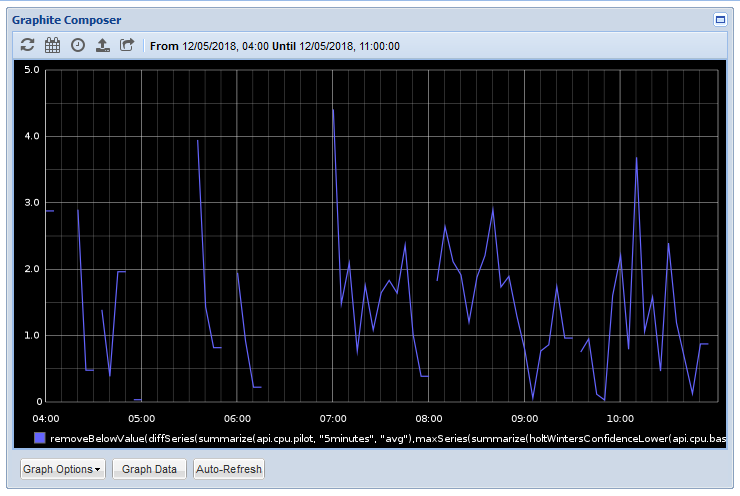
The graph shows us all the times our pilot metric has gone outside the upper CPU threshold and the amount it has violated the bound.

The metric is admittedly somewhat involved so let's breakdown the functions:

Firstly holtWintersConfidenceBands(api.cpu.baseline, 10) will give us 2 metrics representing the upper and lower thresholds based on the data in the api.cpu.baseline metric. It does this up with up to 7 days worth of data in the series to establish the range of values over time. The 10 value we pass in is the delta, the thresholds are multipled based on the delta, the higher the delta, the more lenient the values.

Next summarize(metric, "5minutes", "avg") smooths out the range to an average over 5 minutes. This ensures short spikes are given less precedence and instead trends over time are considered.

As we get 2 metrics back from the confidence bands, we need maxSeries(metric) to get the upper band only. We can use minSeries to get the lower threshold instead.

Then diffSeries(metric1, metric2) will subtract our pilot metric from the threshold. As we are using the upper threshold, if the resulting number is positive it means the metric is higher than the boundary.

Finally removeBelowValue(metric, 0) gets rid of all values under 0 to ensure we are only seeing violations in the graph.

So now we have a graph that shows us only when the pilot box goes over a threshold, we can hook it up to a tool like Seyren to send us an alert when the graph shows any data.

Conclusion

Using a mixture of the built-in Holt-Winters algorithm and a range of helper functions we can quickly set up a way of automating health checks on pilot instances when compared against production.

As the data is a comparison between 2 metrics, rather than a complete prediction, it avoids the common accuracy problem of anomaly detection. This combined with using the delta value gives us a rapid way to adjust the thresholds to reasonable expectations.

This is one of the longest posts I've written (and it took quite some time to put together!) so if you have found it useful please feel free let me know on Twitter at @LukeAMerrett.